Arduino Development with a Raspberry Pi 3

In this article we show how to do Arduino development on an Raspberry Pi 3 with Raspbian. We will describe how to install the GNU GCC tool chain for the AVR microcontroller family, how to compile the archetypal "hello world" program for the Arduino UNO, and how to upload it to an Arduino UNO board.

Introduction

The Arduino UNO is a prototyping board based on the Atmel ATMega328P microcontroller.

The Raspberry Pi is a family of single board computers with ARM based processors. The Raspberry Pi 3 Model B is the latest member of that family (at the time we write this). The Raspberry Pi 3 Model B is quite capable of being used as a desktop development machine. Several Linux distributions are available for the Raspberry Pi. The Raspbian Linux distribution is one of those. Raspbian is based on Debian and is optimized for the Raspberry Pi hardware. Raspbian provides most (all?) of the packages available from the venerable Debian distribution, making it an easy choice for a development system.

In this article we are going to show how you can use a Raspberry Pi 3 installed with Raspbian to develop code intended to be run in an Arduino UNO board. We will do this by going through the steps to create a program for making the Arduino blink a LED. The blinking LED is the archetypal "hello world" program for microcontrollers.

• Blinking LED circuit introduces the circuit diagram for the Arduino with blinking LED. This is a one of the simplest circuits involving an Arduino.
• Installing the GNU GCC tool chain for Arduino shows how to install the tool chain for compiling C code for the Arduino.
• Arduino "hello world" program continues with the instructions for compiling the blinking LED program.
• Uploading the program image to Arduino, finally, shows how to upload the compiled program to the Arduino board.

Please note that in this article we will not be using the Arduino IDE (though it is also available for Raspbian) for writing and compiling our code. We are going to write plain C code and compile it with the GCC cross-compiler for the AVR architecture.

Blinking LED circuit

The "hello world" program for a microcontroller involves making a LED blink. We thus have to prepare the circuit with a LED connected to the Arduino UNO board. The figure below shows the schematic for the circuit that we are going to assemble.

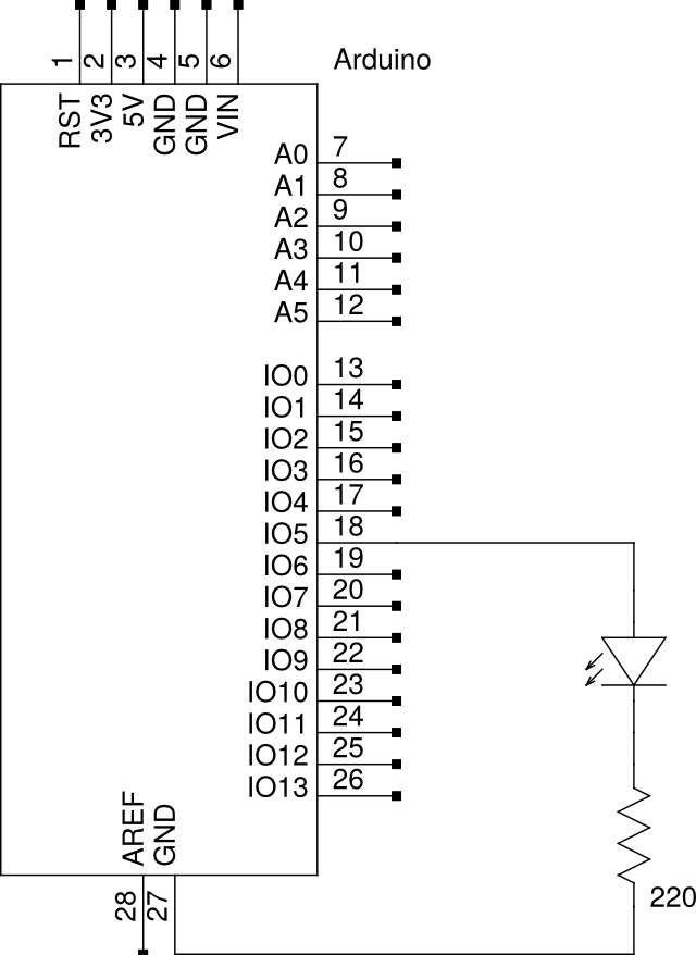
Circuit diagram showing how to connect the LED to the Arduino board.

The circuit diagram above was created with the gschem tool of the gEDA project software suite.

Installing the GNU GCC tool chain for Arduino

The tool chain required for writing C programs for the Arduino is the standard GNU GCC tool chain. This same tool chain can actually be used with the whole Atmel family of AVR microcontrollers. All the required packages are available from the standard Raspbian repositories. We will make use of the following packages:

• gcc-avr - GNU GCC cross compiler for the AVR architecture.
• avr-binutils - GNU Binutils tools for the AVR architecture. These include the GNU linker and other tools for generating the final image files.
• avr-libc - A standard C library for the AVR architecture. This includes the ATMega368p microcontroller of the Arduino UNO.
• avrdude - Tool for uploading program images into the Arduino board.

The procedure for installing the above packages under Raspbian is the familiar one using the apt-get tool. To wit, from a command line:

apt-get install gcc-avr binutils-avr avr-libc avrdude

Now that we have the tools for compiling code, we can continue with actually writing the code in order to compile it.

Arduino "hello world" program

We are now going to write and compile our "hello world" program. As we mentioned before, this will be a program to just make a LED blink in the Arduino board. The full program source code is shown below. The instructions later on will assume we have this code saved in a file unimaginatively named HelloWorld.c.

#include <avr/io.h>
#include <util/delay.h>

const int BLINK_DELAY_MS = 500;

int main(void) {
    /* Set pin 5 of port D for output*/
    DDRD |= _BV(DDD5);

    while (1) {
        /* Set pin 5 of port D high to turn led on */
        PORTD |= _BV(PORTD5);
        _delay_ms(BLINK_DELAY_MS);

        /* Set pin 5 of port D low to turn led off */
        PORTD &= ~_BV(PORTD5);
        _delay_ms(BLINK_DELAY_MS);
    }
    return 0;
}

You will have noticed that the C code makes reference to a pin 5 of port D. The avr-libc library provides a set of functions and macros to interact with the pins from the Atmel AVR microcontroller. In the avr-libc library the pins are named by their native Atmel conventions, and not by their numbering in the Arduino UNO board.

The Arduino documentation describes the pin mapping between the pins in the Atmel AVR processor and the numbering in the Arduino UNO board. From that we see that pin 5 in the Arduino board where we connected our LED (see circuit diagram in Blinking LED circuit) corresponds to pin 5 of port D on the Atmel AVR processor. And it is this pin 5 in port D that we refer to in the C code.

Detailed information on available ports, and how to work with them is available in the ATMega368p data sheet provided by Atmel. Documentation for the avr-libc function and macros used in the program is available on the avr-libc user manual.

We have the source code, we can go ahead and compile it. To compile the code for the Arduino UNO board we will use the GCC cross compiler we installed in the previous section. The commands for compiling the code and producing the final image file are the following:

avr-gcc \
    -DF_CPU=16000000UL -mmcu=atmega328p \
    -o HelloWorld HelloWorld.c
avr-objcopy -O ihex -R .eeprom ./HelloWorld ./HelloWorld.hex

The HelloWorld.hex image file is the final result of compiling the C source code. It is this image file that is used in the next step when uploading the compiled program to the Arduino board.

Uploading the program image to Arduino

Finally we are now going to upload the compiled program to the Arduino board. After uploading the program the Arduino board will automatically start running the program.

In order to upload the program to the Arduino board we first need to connect the board to the host PC with an USB cable. The host PC is, of course, our Raspberry Pi 3 happily running Raspbian.

To upload the code to the Arduino board we need the avrdude tool. The command for uploading the image for the "hello world" program we created in the previous section is the following:

avrdude \
    -c arduino \
    -p ATMEGA328P \
    -P /dev/ttyACM0 \
    -U flash:w:./HelloWorld.hex:i

After the above command completes the program will automatically start running in the Arduino board. The LED should by now be merrily blinking away.

The /dev/ttyACM0 device referenced in the command above is the serial device for communicating with the Arduino board. You can confirm the device path for your specific case by looking into the messages appearing in /var/log/syslog when you connect the Arduino board with the USB cable to the host computer (i.e. your Raspberry Pi 3).

Conclusion

We showed in this article how to prepare a Raspberry Pi 3 with Raspbian to be a development host for Arduino programming. We started with installing the compiler and other development tools. Then we compiled a program for making a LED blink in the Arduino board. And finally we uploaded the program image file to the Arduino board to see it running.

Haskell on CentOS 7

Where we summarily describe how to install the usual Haskell development tools on CentOS 7, and gleefully proceed to compile and run the canonical "hello, world" program.

Introduction

This story begins with us wanting to write Haskell programs.

Functional programming is in the air. From C++ to Java, from Python to Javascript, all your parents usual programming languages have for a while been getting pimped up with functional programming like features. More recent mainstream languages, like Scala or Rust, already addressed functional programming head-on from the start. Of course your grandparents and great-grandparents were also doing it back in the day. So functional programming seems to be one of those good ideas that just take a while to get spread around. Among all the functional programming brouhaha Haskell seems to be getting some increased mind share as of late (at the time we type these words, on the second half of the second decade of the 21^st century AD). So let us assume that all the verbiage we have been spouting is by now enough justification for us to want to know more about Haskell.

The physical act of writing Haskell programs, or for that matter programs in any other language, does not seem to be that difficult. You can do it in your own head. Or by writing it on paper. Or even write it using a computer and your text editor of choice (which, unless you are using cat > myfile.txt to edit your files, will be Emacs, the One True Editor™).

And if writing Haskell programs was all that we wanted our story would then be ended right here, and right now. But we do want more than that. Not only do we want to write Haskell programs, we also want to run those programs! Yes, indeed we are daring and audacious.

Now running Haskell programs, that is a tad little more challenging. Here we will just have to rely on common wisdom regarding how we are to proceed. In order to run Haskell programs we will use a compiler to compile the Haskell source code into an executable. It is that executable that can then be executed (if you pardon the pun), meaning we will then be running the Haskell program.

And that, dear reader — please do allow us to break the fourth wall, and to address you as such — will be the gist of our story. We will endeavor to tell the tale on how to get ourselves an Haskell compiler, and how to compile and run an Haskell program. Humble as this goal may be, we hope it will be a small contribution to keeping us — and you, esteemed reader — on the path to being a better person.

The discerning reader — that would be you, yes, gracious reader — is surely by now wondering why not just ask Google about all this. And oh so right would be that reader of ours. Indeed all the useful information one will get out of this text was procured through the Google search engine. But we want to believe we added value by collating all that information, and presenting it in a clear, straightforward, no-frills way.

Let us continue in earnest with out story. In the following sections we will address three very specific subjects.

• Installing the Haskell development tools on CentOS 7 — These include the Haskell compiler, the magical tool for converting an Haskell source file into an executable.
• Writing and compiling the Haskell "hello, world" program — Here we confirm the Haskell compiler has been installed, and is working as intended.
• Enabling the Emacs mode for Haskell — Your favorite editor (that would be Emacs, yes, we know) obviously includes a mode for editing Haskell source files. Here we describe how to make the Haskell mode available in Emacs (which we do know, we are very mindful of that, is your favorite text editor).

Without further ado let us then continue.

Installing Haskell development tools on CentOS 7

The Haskell development tools are available from the EPEL repository provided by the Fedora Project.

So as very first step we need to configure Yum to include the EPEL repository in the set of repositories used for installing packages. Unless, of course, we had already done it in some distant — or perhaps not — past, being the case that EPEL offers so many usefull packages.

Adding the EPEL repository to Yum has fortunately been made simple by the good people at the Fedora Project. There is a CentOS epel-release package with the express intent of making it simple to configure Yum to use the EPEL repository.

So let us then install said epel-release package. Like this:

[root@localhost ~]# yum install -y epel-release

After the command above completes successfully, the EPEL repository is now part of the set of repositories that Yum uses for fetching packages. And we can now happilly proceed with installing the Haskell development tools.

[root@localhost ~]# yum install -y haskell-platform

Well, that was easy. Let us do a quick check.

jfn@localhost:~$ ghc --version
The Glorious Glasgow Haskell Compilation System, version 7.6.3
jfn@localhost:~$ ghci
GHCi, version 7.6.3: http://www.haskell.org/ghc/  :? for help
Loading package ghc-prim ... linking ... done.
Loading package integer-gmp ... linking ... done.
Loading package base ... linking ... done.
Prelude>

All is cool! Hooray! We did it!

Haskell hello world

We now have the Haskell compiler installed. This means we are ready to create our very first Haskell program. Following the time honored tradition long put in place by our elders, our very first program in a programming language will have to be the canonical "hello, world".

We start with creating the file with the source code. That is easily done using everyone's favorite text editor (that would be Emacs by the way). The source code is shown below. We could have named that file whatever grandiose name we wanted, but having it named hello.hs just sort of feels right.

main = do
  putStrLn "Hello, world!"

With our Haskell source file ready, we need to compile it to generate the executable binary. Let us just do it.

jfn@localhost:~$ ghc --make hello.hs
[1 of 1] Compiling Main             ( hello.hs, hello.o )
Linking hello ...

Finally we have the executable. All that is left is to run it. And run it we will!

jfn@localhost:~$ ./hello
Hello, world!

Wow! Just wow! And with this, gentle reader, we have surely reached one of the high points in this most unpretentious story.

Emacs mode for Haskell

There is an Emacs mode for editing Haskell source code. This Emacs mode provides syntax highlighting and auto-indentation.

A CentOS package is already available that includes this Emacs mode. To install it

[root@localhost ~]# yum install -y emacs-haskell-mode

After installing the above package the Emacs mode works right out of the box. The Haskell mode is automatically activated when opening a file with a .hs extension. Still, one thing you almost surely will want to do is enable the automatic indentation for this mode. To enable automatic indentation just add to the custom-set-variables on your .emacs file the following parameter:

(custom-set-variables
 '(haskell-mode-hook '(turn-on-haskell-indentation)))

Epilogue

And that's it! We are happy campers! Finally ready to tread the flower covered golden path of the Haskell way on our journey to the fabled programming nirvana.

Ilha de Koch

Neste artigo abordaremos resumidamente as figuras geométricas conhecidas como linha de Koch e ilha de Koch. O nome vem do matemático sueco Helge von Koch, que em 1904 referiu num artigo pela primeira vez a curva que é hoje conhecida como linha de Koch.

Linha de Koch

A linha de Koch é uma figura geométrica que nos será útil para definir a ilha de Koch. Consideremos a sequência de figuras que descrevemos em seguida. Partimos de um segmento horizontal, com uma unidade de comprimento.

Ponto de partida para a construção da linha de Koch.

Começamos por dividir este segmento em três partes iguais e substituimos a parte do meio por outros dois segmentos correspondendo a dois lados de um triângulo equilátero. Este passo está ilustrado na figura em baixo. O comprimento de cada um destes 4 segmentos é 1/3 pelo que o comprimento da linha completa é de 4/3.

Primeira iteração da construção da linha de Koch.

No segundo passo fazemos algo semelhante ao realizado no primeiro passo, agora para cada um dos 4 segmentos da figura. Cada segmento é dividido em três e a parte do meio substituida por outros dois segmentos formando dois lados de um triângulo equilátero. Se no primeiro passo a figura era composta por segmentos de comprimento 1/3 agora os segmentos são de comprimento 1/9 e o comprimento total passou a ser 16/9.

Segunda iteração da construção da linha de Koch.

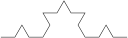
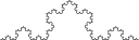
As figuras em baixo correspondem aos passos 3, 4 e 5 deste processo.

Iterações 3, 4 e 5 da construção da linha de Koch.

Continuando com o mesmo procedimento em cada passo, no limite obtém-se a figura designada por linha de Koch. Assumimos, sem demonstração, que existe efectivamente o limite desta sucessão.

A linha de Koch tem, entre outras, as seguintes propriedades interessantes:

• É uma linha contínua.
• Não tem derivada em nenhum ponto. Tomamos aqui a linha como uma aplicação de \(\mathbb{R} \to \mathbb{R}^2\).
• Tem comprimento infinito.

É simples verificar que o comprimento da linha de Koch é infinito. De facto, se chamarmos \(L_n\) ao comprimento da figura do passo \(n\) tem-se que

\[ L_n = \frac{4}{3}L_{n-1} \]

Como \(L_0=1\) então

\[ L_n = \left(\frac{4}{3}\right)^n, \]

que é uma sucessão que cresce sem ter majorante. Ou seja, o comprimento da figura limite é infinito.

Ilha de Koch

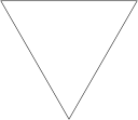
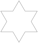
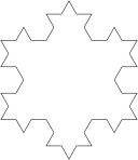
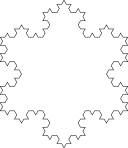
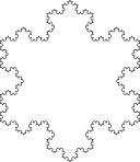
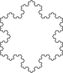
A figura conhecida como ilha de Koch é obtida através de um procedimento semelhante ao usado para criar a linha de Koch, mas em vez de começar com um único segmento começa-se com um triângulo equilátero. As imagens em baixo representam as seis primeiras iterações do procedimento.

A figura inicial e as cinco primeiras iterações da construção da ilha de Koch.

O perímetro da ilha de Koch é infinito. Tal acontece porque esta figura é constituida pela união de três versões idênticas, apropriadamente rodadas e deslocadas, da linha de Koch. No entanto a área da ilha de Koch é claramento limitada. Podemos mesmo calcular a área como o limite da sucessão das áreas das figuras intermédias.

A área da ilha de Koch pode ser obtida como o limite das áreas das figuras intermédias. Vamos então calcular a área \(A_n\) da figura do passo \(n\). A área da figura do passo \(n\) é dada pela soma da área da figura do passo \(n-1\) com as áreas dos pequenos triângulos que são adicionados à figura do passo \(n-1\) para obter a figura do passo \(n\).

Precisamos de saber quantos pequenos triângulos são acrescentados no passo \(n-1\) para obter a figura do passo \(n\). Precisamos também de saber o comprimento do lado desses pequenos triângulos, para calcular a respectiva área.

O número de pequenos triângulos que são acrecentados no passo \(n-1\) corresponde ao número de troços no passo \(n-1\). Chamemos \(c_n\) ao número de troços no passo \(n\). Tem-se então:

\[ c_0=3, \quad c_n=4c_{n-1} \qquad \Rightarrow \qquad c_n = 3\times 4^n \]

O comprimento do lado dos pequenos triângulos que são acrescentados no passo \(n-1\) corresponde ao número de troços que existem no passo \(n\). Chamemos-lhe \(l_n\). Tem-se que:

\[ l_0=1, \quad l_n=\frac{1}{3}l_{n-1} \qquad \Rightarrow \qquad l_n = \left(\frac{1}{3}\right)^n \]

Chamemos \(a_n\) à área de cada um dos pequenos triângulos acrescentados no passo \(n-1\). Sendo a área a de um triângulo equilátero de lado \(l\) dada por \(a=\frac{\sqrt{3}}{4}l^2\) teremos

\[ a_n = \frac{\sqrt{3}}{4} l_n^2 = \frac{\sqrt{3}}{4} \left(\frac{1}{9}\right)^n \]

Com o que já foi dito temos

\[ A_n = A_{n-1} + c_{n-1}a_n \] \[ A_n = A_0 + \sum_{k=1}^n c_{k-1}a_k \] \[ A_n = \frac{\sqrt{3}}{4} \left( 1 + \frac{3}{4} \sum_{k=1}^n \left(\frac{4}{9}\right)^n \right) \]

No limite temos a soma dos termos de uma progressão geométrica de razão \(\frac{4}{9}\). Sendo \(\sum_{k=0}^\infty = \frac{1}{1-r}\), ou \(\sum_{k=1}^\infty = \frac{r}{1-r}\), teremos finalmente a área \(A\) da ilha de Koch como \[ A = \lim A_n = \frac{2\sqrt{3}}{5} \]

Cólofon

As imagens PNG usadas neste artigo com os diferentes passos das iterações da linha de Koch e ilha de Koch foram geradas com Inkscape a partir de ficheiros SVG. Os ficheiros SVG com as figuras foram gerados a partir de um programa para geração de iterações de Sistemas-L escrito na linguagem de scripting Tea.

Cubos Desdobrados

Neste artigo iremos falar de forma muito introdutória sobre poliominós e como se relacionam com dobragens de cubos.

Introdução

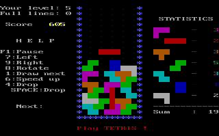
Poliominós são figuras geométricas compostas por quadrados. Cada quadrado é adjacente a um ou mais quadrados pelos lados. O número de quadrados que formam o poliominó corresponde ao seu grau. O jogo Tetris faz uso de poliominós. A imagem em baixo mostra o estado do jogo num instante arbitrário. As peças do jogo são poliominós de grau quatro, ou seja, cada peça é composta por quatro quadrados.

Tetris game screenshot.

Note-se que entre os poliominós do Tetris existem dois pares em que as figuras podem ser obtidas uma da outra através de uma reflexão. As peças B, C e as peças D, E podem ser obtidas uma da outra através de uma reflexão.

Os poliominós de grau quatro que correspondem às peças do jogo Tetris.

Existem duas classes comuns de classificação de poliominós. Poliominós de lado único e poliominós de forma livre.

• Poliominós do lado único --- São poliominós que não podem ser obtidos uns dos outros por qualquer composição de rotações. As figuras do Tetris formam o conjunto dos poliominós de grau quatro de lado único.
• Poliominós de forma livre --- São poliominós que não podem ser obtidos uns dos outros por qualquer composição de rotações e reflexões.

Geração de Poliominós

A geração de poliominós é extremamente simples. Dados os poliominós de grau \(n-1\) podem obter-se todos os poliominós de grau \(n\). O procedimento para a obtenção de todos os poliominós de grau \(n\) é pois recursivo. O processo tem início com o único poliominó de grau 2, formado por dois quadrados.

O procedimento para obtenção dos poliominós de grau \(n\) envolve tratar cada um dos poliominós de grau \(n-1\) da forma descrita em seguida.

Dado um poliominó de grau \(n-1\) são gerados poliominós de grau \(n\) adicionando à figura um novo quadrado em cada uma das posições possíveis. Na imagem em baixo está ilustrado este processamento. A figura cinzenta representa o poliominó original. O quadrado vermelho representa o quadrado que é adicionado à figura original em cada uma das posições possíveis.

Geração de poliominós de grau \(n\) a partir de um poliominó de grau \(n-1\).

Para cada um dos poliominós assim obtidos determina-se se devem ser adicionados à lista de poliominós de grau \(n\) encontrados até ao momento. Para tal verifica-se se o poliominó pode ser obtido de um dos poliominós já encontrados. Se estamos a gerar poliominós de lado único verifica-se se pode ser obtido de rotações. Se estamos a gerar poliominós de forma livre verifica-se se pode ser obtido por uma composição de rotações e reflexão.

Exemplos de Poliominós

Vamos de seguida apresentar os conjuntos de poliominós de forma livre até ao grau 7.

Monominós

Poliominós de grau 1 (monominós) são compostos por um único quadrado. Destes, obviamente, existe apenas um.

Dominós

Existe também apenas um único poliominó de grau 2, composto por dois quadrados.

Triminós

Poliominós de grau 3 são também designados por triminós, dos quais existem apenas 2.

Triminós.

Tetrominós

Os poliominós de grau 4 são as peças do jogo Tetris. Existem 5 na forma livre, visíveis na figura seguinte.

Tetrominós.

Pentominós

Outra designação dos poliominós de grau 5. Existem 12 deles.

Pentominós.

Hexominós

Existem 35 poliominós de grau 6 distintos.

Hexominós.

Heptominós

Existem 108 poliominós de grau 7.

Heptominós.

Dobragens de Cubos

Alguns dos poliominós de grau 6 são dobragens de cubo. Por dobragem de cubo entendemos uma figura que por meio de dobragens apropriadas possa transformar-se num cubo. Cada dobragem individual tem sempre como eixo um lado de um dos quadrados que formam o hexaminó. Não é permitido "rasgar" a figura em qualquer um dos passos das dobragens.

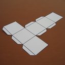
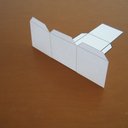
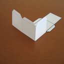
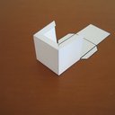
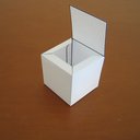
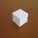
As imagens seguintes ilustram um exemplo da dobragem de um cubo a partir de um hexominó. Cada imagem corresponde a um passo da sequência de dobragens desde a figura plana inicial (o hexominó) até chegar ao cubo.

Os passos da dobragem de um cubo a partir de um hexaminó.

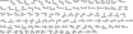
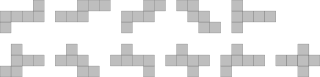
Todos os poliominós de grau 6 de forma livre que correspondem a dobragens de um cubo estão indicados na figura em baixo.

Hexominós que correspondem a dobragens de um cubo.

Estes hexominós foram encontrados inspeccionando visualmente cada um dos 35 hexominós de lado único. A questão que vamos deixar no ar é se existirá algum algoritmo que permita classificar de forma simples um dado hexominó como sendo, ou não, uma dobragem de cubo. Ou, de forma quase equivalente, qual o algoritmo que permite gerar todos os hexominós que são dobragens de um cubo. Esperamos ter resultados para um artigo futuro.

Referências

• Wikipedia:Polyomino.
• Nonius nº 16 - Recensões Críticas de Software.

Cólofon

As imagens PNG usadas neste artigo com figuras de poliominós foram geradas com Inkscape a partir de ficheiros SVG.

Os ficheiros SVG com figuras de poliominós foram gerados a partir de um programa para geração de poliominós escrito na linguagem de scripting Tea.

Triângulo de Sierpinsky

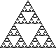
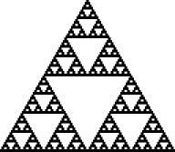
Representação do triângulo de Sierpinski.

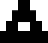
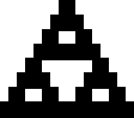
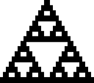
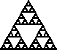
O triângulo de Sierpinsky é um fractal no plano dos reais. Na figura em baixo pode ver-se uma representação do conjunto dos pontos que formam o triângulo de Sierpinski.

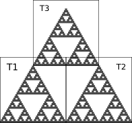
Este conjunto é auto-similar. Por auto-similar entende-se que partes do todo são semelhantes ao todo. Efectivamente, tal como é destacado na figura seguinte, o conjunto completo pode ser obtido através da união de três cópias apropriadamente escaladas e deslocadas do próprio conjunto.

Representação do triângulo de Sierpinski.

Se chamarmos \(S\) ao conjunto dos pontos do triângulo de Sierpinski então podemos dizer que

\[ S = T_1(S) \cup T_2(S) \cup T_3(S) \]

As funções \(T_i : {\mathbb R}^2 \mapsto {\mathbb R}^2\) são transformações afim que realizam os escalamentos e as translações específicos para o triângulo de Sierpinski.

Uma transformação afim tem a forma

\[ Tx = Ax + u \]

onde \(A\) é uma aplicação linear (i. e. corresponde a uma matriz) e o vector \(u\) é uma constante.

No caso do triângulo de Sierpinski as funções \(T_i x = A_i x + u_i\) são caracterizadas da seguinte forma:

\[ A_1 = A_2 = A_3 = \left[ \begin{array}{cc} \frac{1}{2} & 0 \\ 0 & \frac{1}{2} \end{array} \right] \] \[ u_1 = \left[ \begin{array}{c} 0 \\ 0 \end{array} \right] \qquad u_2 = \left[ \begin{array}{c} \frac{1}{2} \\ 0 \end{array} \right] \qquad u_3 = \left[ \begin{array}{c} \frac{1}{4} \\ \frac{\sqrt{3}}{4} \end{array} \right] \]

Existem outras formas de definir o triângulo de Sierpinski. Definamos a função \(F : {\mathbb R}^2 \mapsto {\mathbb R}^2\) como

\[ F(\Lambda) = T_1(\Lambda) \cup T_2(\Lambda) \cup T_3(\Lambda) \]

Então, de acordo com o que tinha atrás já sido exposto temos que o triângulo de Sierpinsky corresponde ao conjunto dos pontos \(S\) onde \(F(S)=S\) Ou seja, o triângulo de Sierpinsky é um ponto fixo da função \(F\). Mas será que existe mesmo um ponto fixo da função \(F\) definida desta forma? Sim, existe. Haveremos noutro artigo de ver com mais detalhe como tal pode ser confirmado. Para já fica a ideia de que a sucessão \[ S_k = F(S_{k-1}), \qquad k \ge 1 \] converge quando o ponto inicial \(S_0\) é um conjunto compacto e desde que a função \(F\) seja uma contração. Esta forma de definir o triângulo de Sierpinsky tem a vantagem de nos permitir criar um procedimento para obter uma aproximação desse conjunto. As figuras seguintes representam os seis primeiros pontos da sucessão \(S_k\) quando o ponto inicial é o quadrado unitário \(S_0 = [0,1] \times [0,1]\).

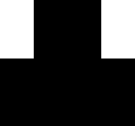
As seis primeiras iterações da construção to Triângulo de Sierpinski.

Estas imagens foram geradas utilizando o Octave. Num futuro artigo veremos como tal foi conseguido.